Note
Go to the end to download the full example code
Quantifying the effects of snow cover#
We classify the effect of snow on a PV system’s DC array. Snow on an array’s modules may reduce string voltage and/or string current, by reducing or blocking irradiance from reaching the cells. These effects may vary across the array since snow cover may not be uniform.
In this analysis, all differences between measured power and power modeled from snow-free irradiance measurements are ascribed to the effects of snow. The effect of snow is classified into one of five categories:
Mode 0: Indicates periods with enough opaque snow that the system is not producing power. Specifically, Mode 0 is when the measured voltage is below the lower bound of the inverter’s MPPT range but the voltage modeled using measured irradiance and ideal transmission is above the lower bound of the inverter’s MPPT range.
Mode 1: Indicates periods when the system has non-uniform snow which affects all strings. Mode 1 is assigned when both operating voltage and current are reduced. Operating voltage is reduced when snow causes mismatch. Current is decreased due to reduced transmission.
Mode 2: Indicates periods when the system has non-uniform snow which affects some strings, causing mismatch for some modules, but not reducing light transmission for other modules.
Mode 3: Indicates periods when the the system has snow that reduces light transmission but doesn’t create mismatch. Operating voltage is consistent with snow-free conditions but current is reduced.
Mode 4: Voltage and current are consistent with snow-free conditions.
Mode -1: Indicates periods when it is unknown if or how snow impacts power output. Mode -1 includes periods when:
Voltage modeled using measured irradiance and ideal transmission is outside the inverter’s MPPT range, OR
Measured voltage exceeds the upper bound of the inverter’s MPPT algorithm.
- The procedure involves four steps:
Model the module’s maximum power current (Imp) and voltage (Vmp) assuming that all the measured POA irradiance reaches the module’s cells.
Use the modeled Imp and measured Imp, determine the fraction of plane-of-array irradiance that reaches the module’s cells. This fraction is called the transmittance.
Model the Vmp that would result from the POA irradiance reduced by the transmittance.
Classify the effect of snow using the ratio of modeled Vmp (from step 3) and measured Vmp.
We demonstrate this analysis using measurements made at the combiner boxes for a utility-scale system.
import pathlib
import pandas as pd
import numpy as np

import pvlib
import matplotlib.pyplot as plt
import matplotlib.dates as mdates
import matplotlib.patches as mpatches
from matplotlib.lines import Line2D

import pvanalytics

# Functions needed for the analysis procedure
from pvanalytics.features import snow

pvanalytics_dir = pathlib.Path(pvanalytics.__file__).parent
Read in 15-minute DC voltage, DC current and AC power data. DC voltage and DC current are measured at the input to the inverter from one combiner box. AC power is measured at the inverter output. Module temperature is collected by a back-of-module sensor. Plane-of-array irradiance data is collected by a heated pyranometer. Data sample was provided by an electric utility. Solar position and other data were added by Sandia to avoid publishing a geographic location.
# Load in utility data
data_file = pvanalytics_dir / 'data' / 'snow_data.csv'
data = pd.read_csv(data_file, index_col='Timestamp', parse_dates=True)

# Explore utility datatset
print('Utility-scale dataset')
print('Start: {}'.format(data.index[0]))
print('End: {}'.format(data.index[-1]))
print('Columns : ' + ', '.join(data.columns))

voltage_col = 'INV1 CB2 Voltage [V]'
power_col = 'INV1 AC Power [kW]'
current_col = 'INV1 CB2 Current [A]'
Utility-scale dataset
Start: 2022-01-05 00:00:00
End: 2022-01-10 23:45:00
Columns : POA [W/m²], INV1 CB2 Voltage [V], INV1 CB2 Current [A], INV1 AC Power [kW], Module Temp [C], Ambient Temp [C], apparent_zenith, zenith, apparent_elevation, elevation, azimuth, equation_of_time, aoi
Retrieve and print system inverter specs and DC electrical configuration
cec_inverter_db = pvlib.pvsystem.retrieve_sam('CECInverter')
my_inverter = cec_inverter_db["Yaskawa_Solectria_Solar__PVI_60TL_480__480V_"]

max_ac_power = my_inverter['Paco']*0.001  # convert from W to kW
mppt_low_voltage = my_inverter['Mppt_low']  # [V]
mppt_high_voltage = my_inverter['Mppt_high']  # [V]

print(f"Inverter AC power rating: {max_ac_power} kW")
print(f"Inverter MPPT range: {mppt_low_voltage} V - {mppt_high_voltage} V")

num_str_per_cb = 4
num_mods_per_str = 18
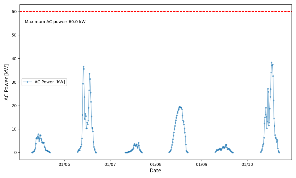
Inverter AC power rating: 60.0 kW
Inverter MPPT range: 540.0 V - 850.0 V
Plot AC power relative to inverter nameplate limits. We are looking for periods of clipping, as these values are outside of MPP operating conditions. In these data, there is no clipping so no need to filter points out.
fig, ax = plt.subplots(figsize=(10, 6))
ax.xaxis.set_major_locator(mdates.DayLocator(interval=1))
ax.xaxis.set_major_formatter(mdates.DateFormatter('%m/%d'))
ax.plot(data[power_col], '.-', alpha=0.5, fillstyle='full',
        label='AC Power [kW]')
ax.axhline(max_ac_power, c='r', ls='--')
ax.text(0.02, max_ac_power - 5, 'Maximum AC power: {} kW'.format(max_ac_power),
        transform=ax.get_yaxis_transform())
ax.set_xlabel('Date', fontsize='large')
ax.set_ylabel('AC Power [kW]', fontsize='large')
ax.legend()
fig.tight_layout()
plt.show()
Model DC voltage and power. Here we use the SAPM. Alternatively, one could use a single diode model.
# SAPM coefficients derived from data from CFV Solar Test Laboratory, 2013.
sapm_coeffs = {
        "Cells_in_Series": 72,
        "Isco": 9.36992857142857,
        "Voco": 46.78626811224489,
        "Impo": 8.895117736670294,
        "Vmpo": 37.88508962264151,
        "Aisc": 0.0002,
        "Aimp": -0.0004,
        "C0": 1.0145,
        "C1": -0.0145,
        "Bvoco": -0.1205,
        "Mbvoc": 0,
        "Bvmpo": -0.1337,
        "Mbvmp": 0,
        "N": 1.0925,
        "C2": -0.4647,
        "C3": -11.900781,
        "FD": 1,
        "A": -3.4247,
        "B": -0.0951,
        "C4": np.nan,
        "C5": np.nan,
        "IXO": np.nan,
        "IXXO": np.nan,
        "C6": np.nan,
        "C7": np.nan,
    }

# Model cell temperature using the SAPM model.

irrad_ref = 1000
data['Cell Temp [C]'] = pvlib.temperature.sapm_cell_from_module(
    data['Module Temp [C]'], data['POA [W/m²]'], deltaT=3)
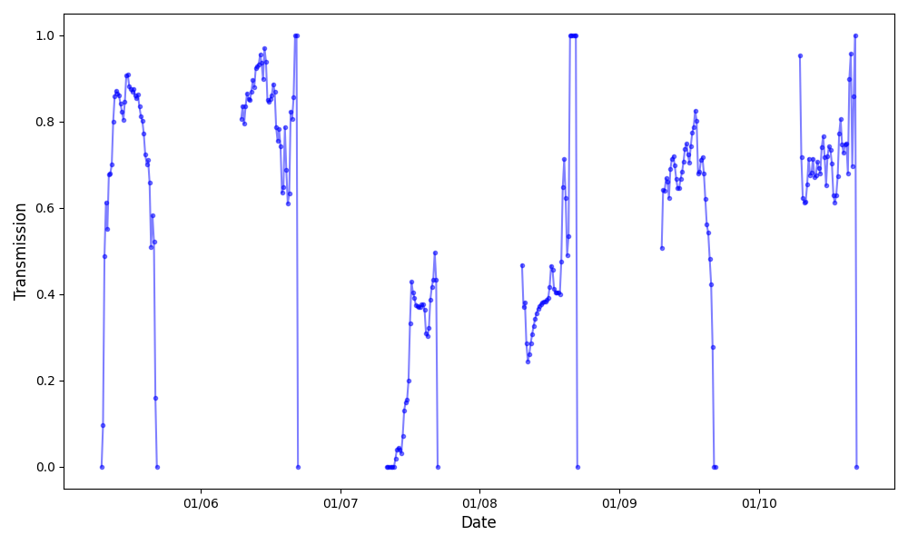
Demonstrate the transmission calculation and plot the result.
# We scale measured current to that of a single string, assuming
# that all strings have the same current.

string_current = data['INV1 CB2 Current [A]'] / num_str_per_cb

# Use SAPM to model effective irradiance from single-string current.


modeled_e_e1 = snow.get_irradiance_sapm(
    data['Cell Temp [C]'], string_current, sapm_coeffs['Impo'],
    sapm_coeffs['C0'], sapm_coeffs['C1'], sapm_coeffs['Aimp'])

T1 = snow.get_transmission(data['POA [W/m²]'], modeled_e_e1, string_current)


fig, ax = plt.subplots(figsize=(10, 6))
date_form = mdates.DateFormatter("%m/%d")
ax.xaxis.set_major_formatter(date_form)

ax.plot(T1, '.-', alpha=0.5, c='b', fillstyle='full')

ax.set_ylabel('Transmission', fontsize='large')
ax.set_xlabel('Date', fontsize='large')
fig.tight_layout()
plt.show()
Visualize measured and modeled DC voltage.
# Model DC output of a single module without the effect of snow.
# Here we use the pyranometer irradiance.
model_no_snow = pvlib.pvsystem.sapm(data['POA [W/m²]'],
                                    data['Cell Temp [C]'],
                                    sapm_coeffs)

# Replaced modeled voltage with NaN when no voltage was measured to make
# comparision between modeled and measured easier.

model_no_snow.loc[data['INV1 CB2 Voltage [V]'].isna(), 'v_mp'] = np.nan

# Scale modeled Vmp to that of a string
modeled_vmp_no_snow = model_no_snow['v_mp'] * num_mods_per_str


# Model DC output of a single module with the effect of snow.
# Here we use the pyranmeter irradiance reduced by the estimated transmission.
model_with_snow = pvlib.pvsystem.sapm(data['POA [W/m²]'] * T1,
                                      data['Cell Temp [C]'],
                                      sapm_coeffs)

# Scale modeled Vmp to that of a string
modeled_vmp_with_snow = model_with_snow['v_mp'] * num_mods_per_str

fig, ax = plt.subplots(figsize=(10, 6))
date_form = mdates.DateFormatter("%H:%M")
ax.xaxis.set_major_formatter(date_form)

ax.plot(modeled_vmp_no_snow, '.-', c='b', fillstyle='full', label='No snow')
ax.plot(modeled_vmp_with_snow, '.-', c='r', fillstyle='full',
        label='With snow')
ax.scatter(data.index, data[voltage_col], s=3, c='k', label='Measured')

ax.xaxis.set_major_locator(mdates.DayLocator(interval=1))
ax.xaxis.set_major_formatter(mdates.DateFormatter('%m/%d'))

ax.axhline(mppt_high_voltage, c='r', ls='--')
ax.text(0.02, mppt_high_voltage - 30,
        'Maximum MPPT voltage: {} V'.format(mppt_high_voltage),
        transform=ax.get_yaxis_transform())
ax.axhline(mppt_low_voltage, c='g', ls='--')
ax.text(0.02, mppt_low_voltage + 20,
        'Minimum MPPT voltage: {} V'.format(mppt_low_voltage),
        transform=ax.get_yaxis_transform())

ax.legend(fontsize='large')
ax.set_ylabel('Voltage [V]', fontsize='large')
ax.set_xlabel('Date', fontsize='large')

fig.tight_layout()
plt.show()

We write a function to assign snow categories, so that we could loop over additional combiner boxes.
def assign_snow_modes(voltage, current, temp_cell, effective_irradiance,
                      coeffs, min_dcv, max_dcv, threshold_vratio,
                      threshold_transmission, num_mods_per_str,
                      num_str_per_cb, temp_ref=25, irrad_ref=1000):

    '''
    Categorizes each data point as Mode 0-4 based on transmission and the
    ratio between measured and modeled votlage.

    This function illustrates a workflow to get to snow mode:

    1. Model effective irradiance based on measured current using the SAPM.
    2. Calculate transmission.
    3. Model voltage from measured irradiance reduced by transmission. Assume
       that all strings are producing voltage.
    4. Determine the snow mode for each point in time.

    Parameters
    ----------
    voltage : array
        Voltage [V] measured at inverter.
    current : array
        Current [A] measured at combiner.
    temp_cell : array
        Cell temperature. [degrees C]
    effective_irradiance : array
        Snow-free POA irradiance measured by a heated pyranometer. [W/m²]
    coeffs : dict
        A dict defining the SAPM parameters, used for pvlib.pvsystem.sapm.
    min_dcv : float
        The lower voltage bound on the inverter's maximum power point
        tracking (MPPT) algorithm. [V]
    max_dcv : numeric
        Upper bound voltage for the MPPT algorithm. [V]
    threshold_vratio : float
        The lower bound on vratio that is found under snow-free conditions,
        determined empirically.
    threshold_transmission : float
        The lower bound on transmission that is found under snow-free
        conditions, determined empirically.
    num_mods_per_str : int
        Number of modules in series in each string.
    num_str_per_cb : int
        Number of strings in parallel at the combiner.

    Returns
    -------
    my_dict : dict
        Keys are ``'transmission'``,
        ``'modeled_voltage_with_calculated_transmission'``,
        ``'modeled_voltage_with_ideal_transmission'``,
        ``'vmp_ratio'``, and ``'mode'``.

        'transmission' is the fracton of POA irradiance that is estimated
        to reach the cells, after being reduced by snow cover.

        'modeled_voltage_with_calculated_transmission' is the Vmp modeled
        with POA irradiance x transmission

        'modeled_voltage_with_ideal_transmission' is the Vmp modeled with
        POA irradiance and assuming transmission is 1.

        'vmp_ratio' is modeled_voltage_with_calculated_transmission divided
        by measured voltage.

        'mode' is the snow mode assigned.
        See :py:func:`pvanalytics.features.snow.categorize`

    '''

    # Calculate transmission
    modeled_e_e = snow.get_irradiance_sapm(
        temp_cell, current / num_str_per_cb, coeffs['Impo'],
        coeffs['C0'], coeffs['C1'], coeffs['Aimp'])

    transmission = snow.get_transmission(effective_irradiance, modeled_e_e,
                                         current / num_str_per_cb)

    # Model voltage for a single module, scale up to array
    modeled_voltage_with_calculated_transmission =\
        pvlib.pvsystem.sapm(effective_irradiance*transmission, temp_cell,
                            coeffs)['v_mp'] * num_mods_per_str
    modeled_voltage_with_ideal_transmission =\
        pvlib.pvsystem.sapm(effective_irradiance, temp_cell,
                            coeffs)['v_mp'] * num_mods_per_str

    mode, vmp_ratio = snow.categorize(
        transmission, voltage, modeled_voltage_with_calculated_transmission,
        modeled_voltage_with_ideal_transmission, min_dcv, max_dcv,
        threshold_vratio, threshold_transmission)

    result = pd.DataFrame(
        index=voltage.index,
        data={
            'transmission': transmission,
            'modeled_voltage_with_calculated_transmission':
                modeled_voltage_with_calculated_transmission,
            'modeled_voltage_with_ideal_transmission':
                modeled_voltage_with_ideal_transmission,
            'vmp_ratio': vmp_ratio,
            'mode': mode})

    return result
Demonstrate transmission, modeled voltage calculation and mode categorization on voltage, current pair.
# threshold_vratio and threshold_transmission were empirically determined
# using data collected on this system over five summers. Transmission and
# vratio were calculated for all data collected in the summer (under the
# assumption that there was no snow present at this time), and histograms
# of the spread of transmission and vratio values were made.
# threshold_vratio is the lower bound on the 95th percentile of all vratios
# calculated for summer data - as in, 95% of all data collected in the summer
# has a vratio that is higher than threshold_vratio. threshold_transmission
# is the same value, but for transmission calculated from data recorded
# during the summer.

threshold_vratio = 0.933
threshold_transmission = 0.598

# Calculate the transmission, model the voltage, and categorize snow mode.
# Use the SAPM to calculate transmission and model the voltage.

inv_cb = 'INV1 CB2'

snow_results = assign_snow_modes(data[voltage_col], data[current_col],
                                 data['Cell Temp [C]'],
                                 data['POA [W/m²]'], sapm_coeffs,
                                 mppt_low_voltage, mppt_high_voltage,
                                 threshold_vratio,
                                 threshold_transmission,
                                 num_mods_per_str,
                                 num_str_per_cb)

# Plot transmission

fig, ax = plt.subplots(figsize=(10, 6))
date_form = mdates.DateFormatter("%m/%d")
ax.xaxis.set_major_formatter(date_form)

ax.plot(snow_results['transmission'], '.-',
        label='INV1 CB2 Transmission')
ax.set_xlabel('Date', fontsize='large')
ax.legend()
fig.tight_layout()
plt.show()

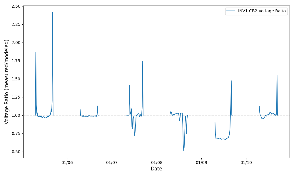
Look at voltage ratio.
fig, ax = plt.subplots(figsize=(10, 6))
date_form = mdates.DateFormatter("%m/%d")
ax.xaxis.set_major_formatter(date_form)

ax.plot(snow_results['vmp_ratio'], label='INV1 CB2 Voltage Ratio')

ax.set_xlabel('Date', fontsize='large')
ax.set_ylabel('Voltage Ratio (measured/modeled)', fontsize='large')
ax.axhline(1, c='k', alpha=0.1, ls='--')
ax.legend()
fig.tight_layout()
plt.show()
Calculate total DC power loss as the difference between modeled and measured power. Total power loss includes losses caused by snow and by other factors, e.g., shading from structures.
model_results = pvlib.pvsystem.sapm(data['POA [W/m²]'],
                                    data['Cell Temp [C]'],
                                    sapm_coeffs)


modeled_power = model_results['p_mp'] * num_str_per_cb * num_mods_per_str
measured_power = data['INV1 CB2 Voltage [V]'] * data['INV1 CB2 Current [A]']
loss_total = np.maximum(modeled_power - measured_power, 0)

# Calculate snow losses. Snow loss occurs when the mode is 0, 1, 2, or 3.
# When the snow loss occurs we assume that all the DC power loss is due to
# snow.
snow_loss_filter = snow_results['mode'].isin([0, 1, 2, 3])
loss_snow = loss_total.copy()
loss_snow[~snow_loss_filter] = 0.0
Plot measured and modeled power, and show snow mode with colored bars.
N = 6
alpha = 0.5
cmap = plt.get_cmap('plasma', N)

fig, ax = plt.subplots(figsize=(10, 6))
date_form = mdates.DateFormatter("%m/%d")
ax.xaxis.set_major_formatter(date_form)
exclude = modeled_power.isna() | snow_results['mode'].isna()
temp = data[~exclude]

# Plot each day individually so we are not exaggerating losses
days_mapped = temp.index.map(lambda x: x.date())
days = np.unique(temp.index.date)
grouped = temp.groupby(temp.index.date)

for d in days:
    temp_grouped = grouped.get_group(d)
    model_power = modeled_power[temp_grouped.index]
    meas_power = measured_power[temp_grouped.index]
    mode = snow_results['mode'][temp_grouped.index]
    ax.plot(model_power, c='k', ls='--')
    ax.plot(meas_power, c='k')
    ax.fill_between(temp_grouped.index, meas_power,
                    model_power, color='k', alpha=alpha)

    chng_pts = np.ravel(np.where(mode.values[:-1]
                                 - mode.values[1:] != 0))

    if len(chng_pts) == 0:
        ax.axvspan(temp_grouped.index[0], temp_grouped.index[-1],
                   color=cmap.colors[mode.at[temp_grouped.index[-1]]],
                   alpha=alpha)
    else:
        set1 = np.append([0], chng_pts)
        set2 = np.append(chng_pts, [-1])

        for start, end in zip(set1, set2):
            my_index = temp_grouped.index[start:end]
            ax.axvspan(
                temp_grouped.index[start], temp_grouped.index[end],
                color=cmap.colors[mode.at[temp_grouped.index[end]]],
                alpha=alpha, ec=None)

# Add different colored intervals to legend
handles, labels = ax.get_legend_handles_labels()

modeled_line = Line2D([0], [0], label='Modeled power', color='k', ls='--')
measured_line = Line2D([0], [0], label='Measured power', color='k')
handles.append(measured_line)
handles.append(modeled_line)

for i in [-1, 0, 1, 2, 3, 4]:  # modes
    color_idx = i + 1
    my_patch = mpatches.Patch(color=cmap.colors[color_idx], label=f'Mode {i}',
                              alpha=alpha)
    handles.append(my_patch)

ax.set_xlabel('Date', fontsize='large')
ax.set_ylabel('DC Power [W]', fontsize='large')
ax.legend(handles=handles, fontsize='large', loc='upper left')
ax.set_title('Snow modes for INV1 CB2',
             fontsize='large')
fig.tight_layout()
plt.show()

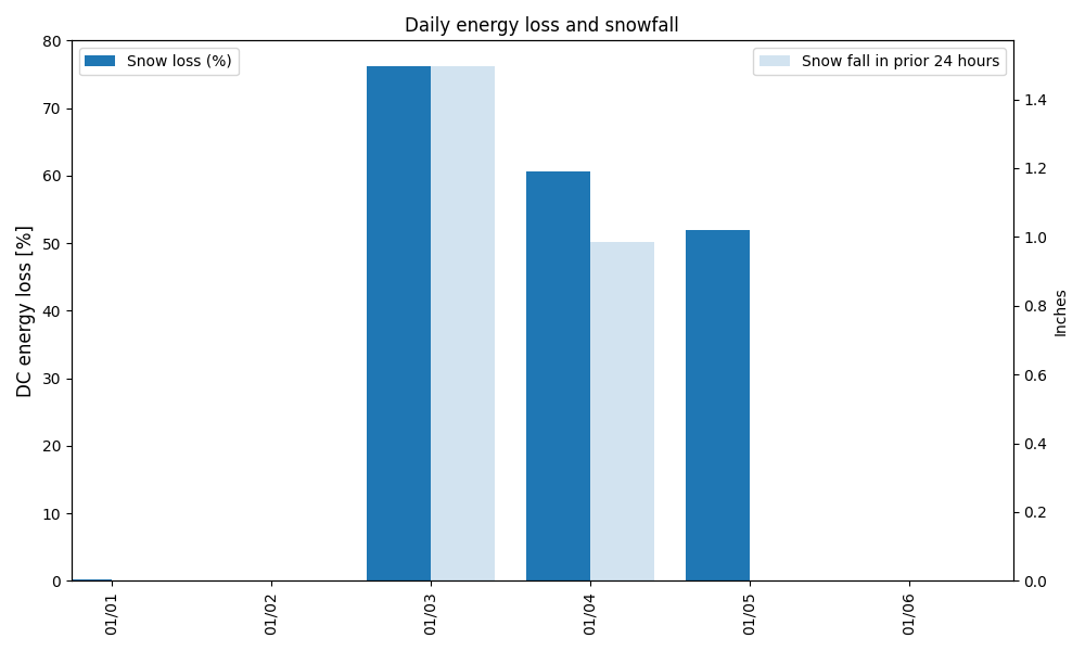
Calculate daily DC energy loss due to snow as a percentage of potential (modeled) DC power.
# DataFrame so that we can group by days.
loss_df = pd.DataFrame(data={'modeled_power': modeled_power,
                             'loss_snow': loss_snow})

# Read in daily snowfall is measured at 7:00 am of each day.
# Daily snowfall will be plotted beside losses, for context.

snowfall_file = pvanalytics_dir / 'data' / 'snow_snowfall.csv'
snowfall = pd.read_csv(snowfall_file, index_col='DATE', parse_dates=True)
snowfall['SNOW'] *= 1/(10*2.54)  # convert from mm depth to inches
snowfall.index = snowfall.index + pd.Timedelta('7H')


days_mapped = loss_df.index.map(lambda x: x.date())
days = np.unique(days_mapped)
loss_df_gped = loss_df.groupby(days_mapped)

snow_loss_daily = pd.Series(index=days, dtype=float)

for d in days:
    temp = loss_df_gped.get_group(d)
    snow_loss_daily.at[d] = 100 * temp['loss_snow'].sum() / \
        temp['modeled_power'].sum()

# Plot daily DC energy loss and daily snowfall totals.
fig, ax = plt.subplots(figsize=(10, 6))
ax2 = ax.twinx()
snow_loss_daily.plot(kind='bar', ax=ax, width=-0.4, align='edge',
                     label='Snow loss (%)')
snowfall['SNOW'].plot(kind='bar', ax=ax2,  width=0.4, alpha=0.2,
                      align='edge',
                      label='Snow fall in prior 24 hours')

ax.legend(loc='upper left')
ax2.legend(loc='upper right')
ax.set_ylabel('DC energy loss [%]', fontsize='large')
ax2.set_ylabel('Inches')
date_form = mdates.DateFormatter("%m/%d")
ax.xaxis.set_major_formatter(date_form)
ax.set_title('Daily energy loss and snowfall', fontsize='large')
fig.tight_layout()
plt.show()
Total running time of the script: (0 minutes 1.803 seconds)