Note
Go to the end to download the full example code
PV Fleets QA Process: Power#
PV Fleets Power QA Pipeline
The NREL PV Fleets Data Initiative uses PVAnalytics routines to assess the quality of systems’ PV data. In this example, the PV Fleets process for assessing the data quality of an AC power data stream is shown. This example pipeline illustrates how several PVAnalytics functions can be used in sequence to assess the quality of a power or energy data stream.
import pandas as pd
import pathlib
from matplotlib import pyplot as plt
import pvanalytics
from pvanalytics.quality import data_shifts as ds
from pvanalytics.quality import gaps
from pvanalytics.quality.outliers import zscore
from pvanalytics.system import (is_tracking_envelope,
                                infer_orientation_fit_pvwatts)
from pvanalytics.features.daytime import power_or_irradiance
from pvanalytics.quality.time import shifts_ruptures
from pvanalytics.features import daytime
import pvlib
from pvanalytics.features.clipping import geometric
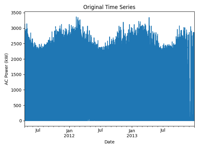
First, we import an AC power data stream from a PV installation at NREL. This data set is publicly available via the PVDAQ database in the DOE Open Energy Data Initiative (OEDI) (https://data.openei.org/submissions/4568), under system ID 50. This data is timezone-localized.
pvanalytics_dir = pathlib.Path(pvanalytics.__file__).parent
file = pvanalytics_dir / 'data' / 'system_50_ac_power_2_full_DST.parquet'
time_series = pd.read_parquet(file)
time_series.set_index('measured_on', inplace=True)
time_series.index = pd.to_datetime(time_series.index)
time_series = time_series['ac_power_2']
latitude = 39.7406
longitude = -105.1775
data_freq = '15min'
time_series = time_series.asfreq(data_freq)
First, let’s visualize the original time series as reference.
time_series.plot(title="Original Time Series")
plt.xlabel("Date")
plt.ylabel("AC Power (kW)")
plt.tight_layout()
plt.show()
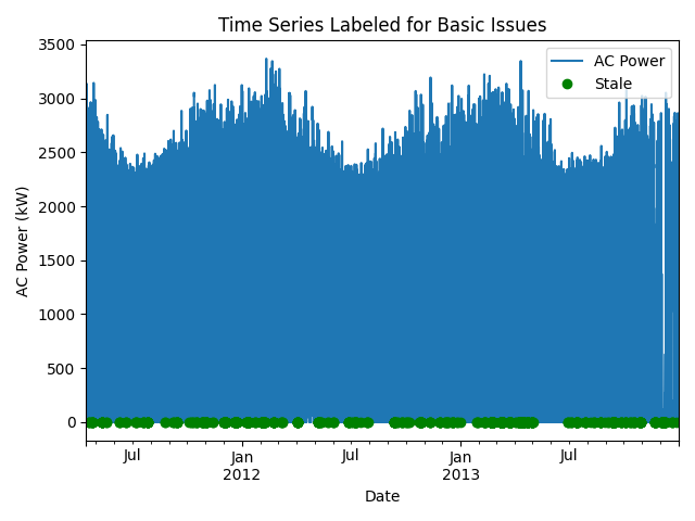
Now, let’s run basic data checks to identify stale and abnormal/outlier data in the time series. Basic data checks include the following steps:
Flatlined/stale data periods (
pvanalytics.quality.gaps.stale_values_round())Negative data
“Abnormal” data periods, which are defined as less than 10% of the daily time series mean
Outliers, which are defined as more than one 4 standard deviations away from the mean (
pvanalytics.quality.outliers.zscore())
# REMOVE STALE DATA (that isn't during nighttime periods)
# Day/night mask
daytime_mask = power_or_irradiance(time_series)
# Stale data mask
stale_data_mask = gaps.stale_values_round(time_series,
                                          window=3,
                                          decimals=2)
stale_data_mask = stale_data_mask & daytime_mask

# REMOVE NEGATIVE DATA
negative_mask = (time_series < 0)

# FIND ABNORMAL PERIODS
daily_min = time_series.resample('D').min()
series_min = 0.1 * time_series.mean()
erroneous_mask = (daily_min >= series_min)
erroneous_mask = erroneous_mask.reindex(index=time_series.index,
                                        method='ffill',
                                        fill_value=False)

# FIND OUTLIERS (Z-SCORE FILTER)
zscore_outlier_mask = zscore(time_series, zmax=4,
                             nan_policy='omit')

# Get the percentage of data flagged for each issue, so it can later be logged
pct_stale = round((len(time_series[
    stale_data_mask].dropna())/len(time_series.dropna())*100), 1)
pct_negative = round((len(time_series[
    negative_mask].dropna())/len(time_series.dropna())*100), 1)
pct_erroneous = round((len(time_series[
    erroneous_mask].dropna())/len(time_series.dropna())*100), 1)
pct_outlier = round((len(time_series[
    zscore_outlier_mask].dropna())/len(time_series.dropna())*100), 1)

# Visualize all of the time series issues (stale, abnormal, outlier, etc)
time_series.plot()
labels = ["AC Power"]
if any(stale_data_mask):
    time_series.loc[stale_data_mask].plot(ls='', marker='o', color="green")
    labels.append("Stale")
if any(negative_mask):
    time_series.loc[negative_mask].plot(ls='', marker='o', color="orange")
    labels.append("Negative")
if any(erroneous_mask):
    time_series.loc[erroneous_mask].plot(ls='', marker='o', color="yellow")
    labels.append("Abnormal")
if any(zscore_outlier_mask):
    time_series.loc[zscore_outlier_mask].plot(
        ls='', marker='o', color="purple")
    labels.append("Outlier")
plt.legend(labels=labels)
plt.title("Time Series Labeled for Basic Issues")
plt.xlabel("Date")
plt.ylabel("AC Power (kW)")
plt.tight_layout()
plt.show()
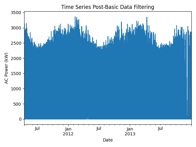
Now, let’s filter out any of the flagged data from the basic power checks (stale or abnormal data). Then we can re-visualize the data post-filtering.
# Filter the time series, taking out all of the issues
issue_mask = ((~stale_data_mask) & (~negative_mask) &
              (~erroneous_mask) & (~zscore_outlier_mask))

time_series = time_series[issue_mask]
time_series = time_series.asfreq(data_freq)

# Visualize the time series post-filtering
time_series.plot(title="Time Series Post-Basic Data Filtering")
plt.xlabel("Date")
plt.ylabel("AC Power (kW)")
plt.tight_layout()
plt.show()
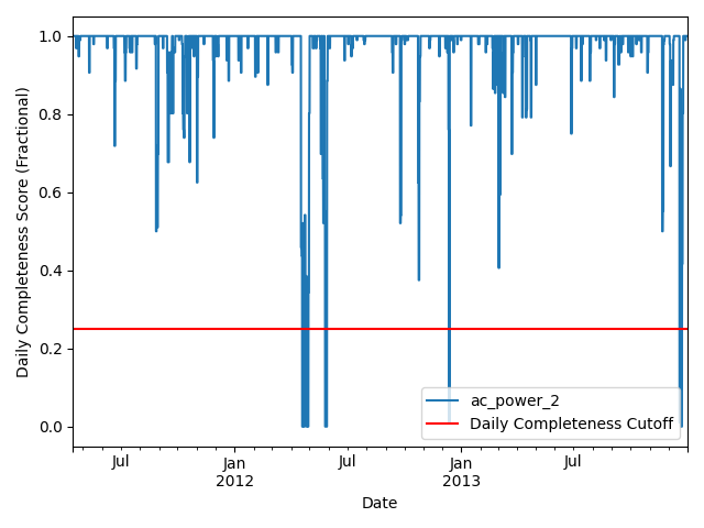
We filter the time series based on its daily completeness score. This filtering scheme requires at least 25% of data to be present for each day to be included. We further require at least 10 consecutive days meeting this 25% threshold to be included.
# Visualize daily data completeness
data_completeness_score = gaps.completeness_score(time_series)

# Visualize data completeness score as a time series.
data_completeness_score.plot()
plt.xlabel("Date")
plt.ylabel("Daily Completeness Score (Fractional)")
plt.axhline(y=0.25, color='r', linestyle='-',
            label='Daily Completeness Cutoff')
plt.legend()
plt.tight_layout()
plt.show()

# Trim the series based on daily completeness score
trim_series = pvanalytics.quality.gaps.trim_incomplete(
    time_series, minimum_completeness=.25, freq=data_freq)
first_valid_date, last_valid_date = \
    pvanalytics.quality.gaps.start_stop_dates(trim_series)
time_series = time_series[first_valid_date.tz_convert(time_series.index.tz):
                          last_valid_date.tz_convert(time_series.index.tz)]
time_series = time_series.asfreq(data_freq)
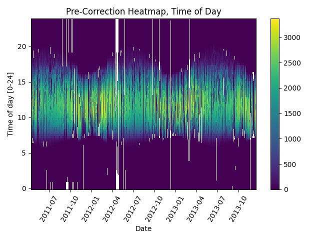
Next, we check the time series for any time shifts, which may be caused by
time drift or by incorrect time zone assignment. To do this, we compare
the modelled midday time for the particular system location to its
measured midday time. We use
pvanalytics.quality.gaps.stale_values_round()) to determine the
presence of time shifts in the series.
# Plot the heatmap of the AC power time series before time shift correction.
plt.figure()
# Get time of day from the associated datetime column
time_of_day = pd.Series(time_series.index.hour +
time_series.index.minute/60,
index=time_series.index)
# Pivot the dataframe
dataframe = pd.DataFrame(pd.concat([time_series, time_of_day], axis=1))
dataframe.columns = ["values", 'time_of_day']
dataframe = dataframe.dropna()
dataframe_pivoted = dataframe.pivot_table(index='time_of_day',
columns=dataframe.index.date,
values="values")
plt.pcolormesh(dataframe_pivoted.columns,
dataframe_pivoted.index,
dataframe_pivoted,
shading='auto')
plt.ylabel('Time of day [0-24]')
plt.xlabel('Date')
plt.xticks(rotation=60)
plt.title('Pre-Correction Heatmap, Time of Day')
plt.colorbar()
plt.tight_layout()
plt.show()
# Get the modeled sunrise and sunset time series based on the system's
# latitude-longitude coordinates
modeled_sunrise_sunset_df = pvlib.solarposition.sun_rise_set_transit_spa(
time_series.index, latitude, longitude)
# Calculate the midday point between sunrise and sunset for each day
# in the modeled irradiance series
modeled_midday_series = modeled_sunrise_sunset_df['sunrise'] + \
(modeled_sunrise_sunset_df['sunset'] -
modeled_sunrise_sunset_df['sunrise']) / 2
# Run day-night mask on the irradiance time series
daytime_mask = power_or_irradiance(time_series,
freq=data_freq,
low_value_threshold=.005)
# Generate the sunrise, sunset, and halfway points for the data stream
sunrise_series = daytime.get_sunrise(daytime_mask)
sunset_series = daytime.get_sunset(daytime_mask)
midday_series = sunrise_series + ((sunset_series - sunrise_series)/2)
# Convert the midday and modeled midday series to daily values
midday_series_daily, modeled_midday_series_daily = (
midday_series.resample('D').mean(),
modeled_midday_series.resample('D').mean())
# Set midday value series as minutes since midnight, from midday datetime
# values
midday_series_daily = (midday_series_daily.dt.hour * 60 +
midday_series_daily.dt.minute +
midday_series_daily.dt.second / 60)
modeled_midday_series_daily = \
(modeled_midday_series_daily.dt.hour * 60 +
modeled_midday_series_daily.dt.minute +
modeled_midday_series_daily.dt.second / 60)
# Estimate the time shifts by comparing the modelled midday point to the
# measured midday point.
is_shifted, time_shift_series = shifts_ruptures(modeled_midday_series_daily,
midday_series_daily,
period_min=15,
shift_min=15,
zscore_cutoff=1.5)
# Create a midday difference series between modeled and measured midday, to
# visualize time shifts. First, resample each time series to daily frequency,
# and compare the data stream's daily halfway point to the modeled halfway
# point
midday_diff_series = (modeled_midday_series.resample('D').mean() -
midday_series.resample('D').mean()
).dt.total_seconds() / 60
# Generate boolean for detected time shifts
if any(time_shift_series != 0):
time_shifts_detected = True
else:
time_shifts_detected = False
# Build a list of time shifts for re-indexing. We choose to use dicts.
time_shift_series.index = pd.to_datetime(
time_shift_series.index)
changepoints = (time_shift_series != time_shift_series.shift(1))
changepoints = changepoints[changepoints].index
changepoint_amts = pd.Series(time_shift_series.loc[changepoints])
time_shift_list = list()
for idx in range(len(changepoint_amts)):
if idx < (len(changepoint_amts) - 1):
time_shift_list.append({"datetime_start":
str(changepoint_amts.index[idx]),
"datetime_end":
str(changepoint_amts.index[idx + 1]),
"time_shift": changepoint_amts[idx]})
else:
time_shift_list.append({"datetime_start":
str(changepoint_amts.index[idx]),
"datetime_end":
str(time_shift_series.index.max()),
"time_shift": changepoint_amts[idx]})
# Correct any time shifts in the time series
new_index = pd.Series(time_series.index, index=time_series.index)
for i in time_shift_list:
new_index[(time_series.index >= pd.to_datetime(i['datetime_start'])) &
(time_series.index < pd.to_datetime(i['datetime_end']))] = \
time_series.index + pd.Timedelta(minutes=i['time_shift'])
time_series.index = new_index
# Remove duplicated indices and sort the time series (just in case)
time_series = time_series[~time_series.index.duplicated(
keep='first')].sort_index()
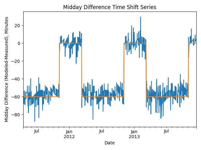
# Plot the difference between measured and modeled midday, as well as the
# CPD-estimated time shift series.
plt.figure()
midday_diff_series.plot()
time_shift_series.plot()
plt.title("Midday Difference Time Shift Series")
plt.xlabel("Date")
plt.ylabel("Midday Difference (Modeled-Measured), Minutes")
plt.tight_layout()
plt.show()
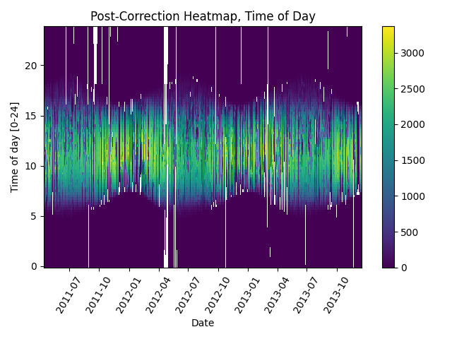
# Plot the heatmap of the irradiance time series
plt.figure()
# Get time of day from the associated datetime column
time_of_day = pd.Series(time_series.index.hour +
time_series.index.minute/60,
index=time_series.index)
# Pivot the dataframe
dataframe = pd.DataFrame(pd.concat([time_series, time_of_day], axis=1))
dataframe.columns = ["values", 'time_of_day']
dataframe = dataframe.dropna()
dataframe_pivoted = dataframe.pivot_table(index='time_of_day',
columns=dataframe.index.date,
values="values")
plt.pcolormesh(dataframe_pivoted.columns,
dataframe_pivoted.index,
dataframe_pivoted,
shading='auto')
plt.ylabel('Time of day [0-24]')
plt.xlabel('Date')
plt.xticks(rotation=60)
plt.title('Post-Correction Heatmap, Time of Day')
plt.colorbar()
plt.tight_layout()
plt.show()
Next, we check the time series for any abrupt data shifts. We take the
longest continuous part of the time series that is free of data shifts.
We use pvanalytics.quality.data_shifts.detect_data_shifts() to
detect data shifts in the time series.
# Resample the time series to daily mean
time_series_daily = time_series.resample('D').mean()
data_shift_start_date, data_shift_end_date = \
    ds.get_longest_shift_segment_dates(time_series_daily)
data_shift_period_length = (data_shift_end_date -
                            data_shift_start_date).days

# Get the number of shift dates
data_shift_mask = ds.detect_data_shifts(time_series_daily)
# Get the shift dates
shift_dates = list(time_series_daily[data_shift_mask].index)
if len(shift_dates) > 0:
    shift_found = True
else:
    shift_found = False

# Visualize the time shifts for the daily time series
print("Shift Found: ", shift_found)
edges = ([time_series_daily.index[0]] + shift_dates +
         [time_series_daily.index[-1]])
fig, ax = plt.subplots()
for (st, ed) in zip(edges[:-1], edges[1:]):
    ax.plot(time_series_daily.loc[st:ed])
plt.title("Daily Time Series Labeled for Data Shifts")
plt.xlabel("Date")
plt.ylabel("Mean Daily AC Power (kW)")
plt.tight_layout()
plt.show()
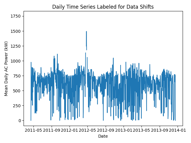
Shift Found: False
Use logic-based and ML-based clipping functions to identify clipped periods in the time series data, and plot the filtered data.
# REMOVE CLIPPING PERIODS
clipping_mask = geometric(ac_power=time_series,
                          freq=data_freq)

# Get the pct clipping
clipping_mask.dropna(inplace=True)
pct_clipping = round(100*(len(clipping_mask[
    clipping_mask])/len(clipping_mask)), 4)
if pct_clipping >= 0.5:
    clipping = True
    clip_pwr = time_series[clipping_mask].median()
else:
    clipping = False
    clip_pwr = None

if clipping:
    # Plot the time series with clipping labeled
    time_series.plot()
    time_series.loc[clipping_mask].plot(ls='', marker='o')
    plt.legend(labels=["AC Power", "Clipping"],
               title="Clipped")
    plt.title("Time Series Labeled for Clipping")
    plt.xticks(rotation=20)
    plt.xlabel("Date")
    plt.ylabel("AC Power (kW)")
    plt.tight_layout()
    plt.show()
    plt.close()
else:
    print("No clipping detected!!!")
No clipping detected!!!
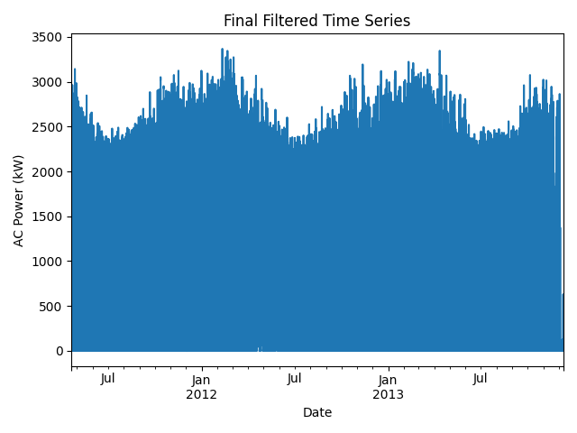
We filter the time series to only include the longest shift-free period. We then visualize the final time series post-QA filtering.
time_series = time_series[
    (time_series.index >=
     data_shift_start_date.tz_convert(time_series.index.tz)) &
    (time_series.index <=
     data_shift_end_date.tz_convert(time_series.index.tz))]

time_series = time_series.asfreq(data_freq)

# Plot the final filtered time series.
time_series.plot(title="Final Filtered Time Series")
plt.xlabel("Date")
plt.ylabel("AC Power (kW)")
plt.tight_layout()
plt.show()
Estimate the azimuth and tilt of the system, based on the power series data. The ground truth azimuth and tilt for this system are 158 and 45 degrees, respectively.
# Import the PSM3 data. This data is pulled via the following function in
# PVLib: :py:func:`pvlib.iotools.get_psm3`
file = pvanalytics_dir / 'data' / 'system_50_ac_power_2_full_DST_psm3.parquet'
psm3 = pd.read_parquet(file)
psm3.set_index('index', inplace=True)
psm3.index = pd.to_datetime(psm3.index)

psm3 = psm3.reindex(pd.date_range(psm3.index[0],
                                  psm3.index[-1],
                                  freq=data_freq)).interpolate()
psm3.index = psm3.index.tz_convert(time_series.index.tz)
psm3 = psm3.reindex(time_series.index)
is_clear = (psm3.ghi_clear == psm3.ghi)
is_daytime = (psm3.ghi > 0)

# Trim based on clearsky and daytime values
time_series_clearsky = time_series.reindex(is_daytime.index)[
    (is_clear) & (is_daytime)].dropna()

# Get final PSM3 data
psm3_clearsky = psm3.loc[time_series_clearsky.index]
solpos_clearsky = pvlib.solarposition.get_solarposition(
    time_series_clearsky.index, latitude, longitude)

# Estimate the azimuth and tilt using PVWatts-based method
predicted_tilt, predicted_azimuth, r2 = infer_orientation_fit_pvwatts(
    time_series_clearsky,
    psm3_clearsky.ghi_clear,
    psm3_clearsky.dhi_clear,
    psm3_clearsky.dni_clear,
    solpos_clearsky.zenith,
    solpos_clearsky.azimuth,
    temperature=psm3_clearsky.temp_air,
    azimuth_min=90,
    azimuth_max=275)

print("Predicted azimuth: " + str(predicted_azimuth))
print("Predicted tilt: " + str(predicted_tilt))
Predicted azimuth: 161.27396222501486
Predicted tilt: 42.20903060025887
Look at the daily power profile for summer and winter months, and identify if the data stream is associated with a fixed-tilt or single-axis tracking system.
# CHECK MOUNTING CONFIGURATION
daytime_mask = power_or_irradiance(time_series)
predicted_mounting_config = is_tracking_envelope(
    time_series,
    daytime_mask,
    clipping_mask.reindex(index=time_series.index))

print("Predicted Mounting configuration:")
print(predicted_mounting_config.name)
Predicted Mounting configuration:
FIXED
Generate a dictionary output for the QA assessment of this data stream, including the percent stale and erroneous data detected, any shift dates, time shift dates, clipping information, and estimated mounting configuration.
qa_check_dict = {"original_time_zone_offset": time_series.index.tz,
                 "pct_stale": pct_stale,
                 "pct_negative": pct_negative,
                 "pct_erroneous": pct_erroneous,
                 "pct_outlier": pct_outlier,
                 "time_shifts_detected": time_shifts_detected,
                 "time_shift_list": time_shift_list,
                 "data_shifts": shift_found,
                 "shift_dates": shift_dates,
                 "clipping": clipping,
                 "clipping_threshold": clip_pwr,
                 "pct_clipping": pct_clipping,
                 "mounting_config": predicted_mounting_config.name,
                 "predicted_azimuth": predicted_azimuth,
                 "predicted_tilt": predicted_tilt}

print("QA Results:")
print(qa_check_dict)
QA Results:
{'original_time_zone_offset': pytz.FixedOffset(-420), 'pct_stale': 0.7, 'pct_negative': 0.0, 'pct_erroneous': 0.0, 'pct_outlier': 0.0, 'time_shifts_detected': True, 'time_shift_list': [{'datetime_start': '2011-04-15 00:00:00-07:00', 'datetime_end': '2011-11-06 00:00:00-07:00', 'time_shift': -60.0}, {'datetime_start': '2011-11-06 00:00:00-07:00', 'datetime_end': '2012-03-11 00:00:00-07:00', 'time_shift': 0.0}, {'datetime_start': '2012-03-11 00:00:00-07:00', 'datetime_end': '2012-11-04 00:00:00-07:00', 'time_shift': -60.0}, {'datetime_start': '2012-11-04 00:00:00-07:00', 'datetime_end': '2013-03-10 00:00:00-07:00', 'time_shift': 0.0}, {'datetime_start': '2013-03-10 00:00:00-07:00', 'datetime_end': '2013-11-03 00:00:00-07:00', 'time_shift': -60.0}, {'datetime_start': '2013-11-03 00:00:00-07:00', 'datetime_end': '2013-12-17 00:00:00-07:00', 'time_shift': 0.0}], 'data_shifts': False, 'shift_dates': [], 'clipping': False, 'clipping_threshold': None, 'pct_clipping': 0.0842, 'mounting_config': 'FIXED', 'predicted_azimuth': 161.27396222501486, 'predicted_tilt': 42.20903060025887}
Total running time of the script: (0 minutes 23.640 seconds)